Neural Networks 101: A Mathematical Deep Dive for Developers (2025)

To the uninitiated, "Deep Learning" often sounds like arcane magic—a black box that ingests data and spits out intelligence. To the initiated, however, it is simply Matrix Multiplication and Calculus scaling to massive proportions.

As software developers, we are accustomed to deterministic logic: if x > 5 then y. Neural Networks fundamentally differ because they are Probabilistic and Continual. They are not explicitly programmed with rules; they are optimized to find patterns.

In this guide, we will banish the "Black Box" mentality. Instead of jumping straight into high-level libraries like TensorFlow or PyTorch, we will start with a blank Python file and the fundamental mathematics that underpin the AI revolution. By the end, you will understand exactly what models like ChatGPT are doing at the atomic level when they "think."

Part 1: The Perceptron (The Atom of AI)

The fundamental unit of a neural network is the Neuron (or Perceptron). It is loosely inspired by biology, but distinct.

1.1 Anatomy of a Neuron

A single neuron does a simple job:

Takes multiple Inputs ($x_1, x_2, ...$).
Multiplies them by Weights ($w_1, w_2, ...$).
Adds a Bias ($b$).
Sums them up ($z$).
Passes the sum through an Activation Function ($\sigma$) to get the Output ($a$).

Mathematically: $$ z = (x_1 \cdot w_1) + (x_2 \cdot w_2) + ... + b $$ $$ z = \sum (x_i \cdot w_i) + b $$ $$ y = \sigma(z) $$

1.2 The Intuition

Think of it as a decision-making process. Decision: Should I go to the beach?

Inputs:

Is it sunny? ($x_1 = 1$)
Do I have free time? ($x_2 = 1$)
Is my car broken? ($x_3 = 0$)

Weights (Importance):

Sunniness is important ($w_1 = 5$)
Free time is crucial ($w_2 = 10$)
Broken car is a dealbreaker ($w_3 = -20$)

Bias (Threshold):

I generally like the beach ($b = 2$)

Calculation: $$ z = (1 \cdot 5) + (1 \cdot 10) + (0 \cdot -20) + 2 $$ $$ z = 17 $$

Output: If our activation function is a simple step (if $z > 0$, return 1), then YES, go to the beach.

The "Learning" part of Machine Learning is simply finding the best numbers for $w$ and $b$ so the neuron makes the "right" decision as often as possible.

Part 2: Activation Functions (The Spark)

Without activation functions, a neural network is just a Linear Regression model. No matter how many layers you stack, it can only solve linear problems. Non-linearity allows it to learn complex patterns (curves, shapes, logic).

2.1 The Classics

Sigmoid: S-shaped curve. Squeezes output between 0 and 1. $$ \sigma(x) = \frac{1}{1 + e^{-x}} $$ Problem: Vanishing Gradient (derivatives get tiny at the edges).
Tanh: Squeezes between -1 and 1. Problem: Still suffers from Vanishing Gradient.

2.2 The Modern Standard

ReLU (Rectified Linear Unit): $$ f(x) = \max(0, x) $$ If positive, pass it through. If negative, output zero. Why basic?: It's computationally free. It solves vanishing gradients for positive numbers. It works unreasonably well. Problem: "Dead ReLUs" (if a neuron gets stuck in the negative zone, it never recovers).
Leaky ReLU: Allows a small gradient when negative ($0.01x$). Keeps neurons alive.
GELU / Swish: Smoother versions of ReLU used in Transformers (GPT, BERT).

Part 3: Example Implementation (NumPy)

Let's code a single neuron in Python without libraries.

import numpy as np

class Neuron:
    def __init__(self, num_inputs):
        # Initialize weights randomly, bias to 0
        self.weights = np.random.randn(num_inputs)
        self.bias = 0.0

    def sigmoid(self, x):
        return 1 / (1 + np.exp(-x))

    def forward(self, inputs):
        # Dot product: (i1*w1) + (i2*w2) + ...
        z = np.dot(inputs, self.weights) + self.bias
        return self.sigmoid(z)

# Test it
neuron = Neuron(3)
inputs = np.array([1, 0, 5])
output = neuron.forward(inputs)
print(f"Output: {output:.4f}")

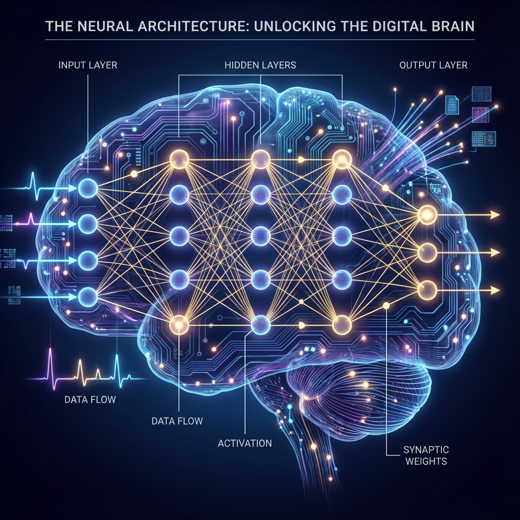
Part 4: The Network (The Crowd)

One neuron is weak. A network of them is powerful. We organize them into Layers.

Input Layer: Receives raw data (pixels of an image, words of a sentence).
Hidden Layers: The "Black Box". They extract features.
- Layer 1 might detect "edges".
- Layer 2 might detect "shapes".
- Layer 3 might detect "eyes".
Output Layer: Final prediction (Cat vs Dog).

The Matrix View

We don't loop over neurons. We use Linear Algebra. If we have 3 inputs and a layer of 4 neurons, our weights are a $3 \times 4$ matrix.

$$ Output = Activation(Input \cdot Weights + Bias) $$

This allows GPUs to parallelize millions of operations.

Part 5: The Loss Function (The Scoreboard)

How do we know if the network is doing a good job? We measure the Loss (Error).

MSE (Mean Squared Error): Used for Regression (predicting prices). $$ Loss = (Predicted - Actual)^2 $$
Cross-Entropy Loss: Used for Classification (Cat vs Dog). measures the distance between probability distributions.

Goal: Minimize the Loss. It is an optimization problem. Imagine a hiker (the algorithm) trying to find the lowest valley (min loss) in a mountain range (the weight landscape) while blindfolded.

Part 6: Backpropagation (The Magic)

This is the hardest part. How does the network learn? How do we know which specific weight to change, and by how much?

We use The Chain Rule from Calculus.

If $Loss$ depends on $Output$, and $Output$ depends on $Weight$, then: $$ \frac{\partial Loss}{\partial Weight} = \frac{\partial Loss}{\partial Output} \cdot \frac{\partial Output}{\partial Weight} $$

This is the Gradient. It tells us: "If you increase this weight by a tiny bit, the loss will go up/down by this much."

Algorithm:

Forward Pass: Input -> Hidden -> Output -> Calculate Loss.
Backward Pass: Calculate gradients from Output back to Input.
Update: Nudge weights in the opposite direction of the gradient.

$$ w*{new} = w*{old} - (LearningRate \cdot Gradient) $$

Part 7: Building a Neural Network from Scratch

Let's solve the famous XOR problem. (0,0)->0, (0,1)->1, (1,0)->1, (1,1)->0. Linear models cannot solve this. We need a hidden layer.

import numpy as np

# 1. Data (XOR)
X = np.array([[0,0], [0,1], [1,0], [1,1]])
y = np.array([[0], [1], [1], [0]])

# 2. Architecture
input_size = 2
hidden_size = 4
output_size = 1
learning_rate = 0.1

# 3. Initialize Weights
# Layer 1 weights (2x4)
W1 = np.random.randn(input_size, hidden_size)
b1 = np.zeros((1, hidden_size))
# Layer 2 weights (4x1)
W2 = np.random.randn(hidden_size, output_size)
b2 = np.zeros((1, output_size))

def sigmoid(x):
    return 1 / (1 + np.exp(-x))

def sigmoid_derivative(x):
    return x * (1 - x)

# 4. Training Loop
for epoch in range(10000):
    # --- Forward Pass ---
    # Layer 1
    hidden_input = np.dot(X, W1) + b1
    hidden_output = sigmoid(hidden_input)

    # Layer 2
    final_input = np.dot(hidden_output, W2) + b2
    final_output = sigmoid(final_input)

    # --- Loss (MSE) ---
    loss = np.mean(np.square(y - final_output))

    if epoch % 1000 == 0:
        print(f"Epoch {epoch}, Loss: {loss:.4f}")

    # --- Backpropagation ---
    # Calculate error at output
    error = y - final_output
    # How much did final layer contribute to error?
    d_output = error * sigmoid_derivative(final_output)

    # Propagate error to hidden layer
    error_hidden = d_output.dot(W2.T)
    d_hidden = error_hidden * sigmoid_derivative(hidden_output)

    # --- Update Weights (Gradient Descent) ---
    W2 += hidden_output.T.dot(d_output) * learning_rate
    b2 += np.sum(d_output, axis=0, keepdims=True) * learning_rate
    W1 += X.T.dot(d_hidden) * learning_rate
    b1 += np.sum(d_hidden, axis=0, keepdims=True) * learning_rate

# 5. Prediction
print("\nPredictions:")
print(final_output)

If you run this, the loss drops to near zero. The network "learned" XOR.

Part 8: Optimization Algorithms (The Hiker's Strategy)

In the example above, we uses plain SGD (Stochastic Gradient Descent). But the mountain range is treacherous (saddle points, local minima).

Momentum: Imagine the hiker is a heavy ball. It gains speed. If gradients are noisy, momentum keeps it moving in the right general direction.
RMSprop: Adapts the learning rate. If a weight has steep gradients, slow down. If flat, speed up.
Adam (Adaptive Moment Estimation): Strategies 1 + 2 combined. It creates a custom learning rate for every single parameter.
- It is the default optimizer for almost everything today.
- AdamW: Adam with "Weight Decay" (a form of regularization) fixed. This is what GPT models use.

Part 9: Modern Architectures

We started with Dense (Fully Connected) layers. But they aren't efficiently for images or text.

9.1 CNNs (Convolutional Neural Networks)

For Images. Instead of connecting every pixel to every neuron, we use Filters (kernels). A $3 \times 3$ filter slides over the image (Convolution) to detect features like vertical lines. This is "Translation Invariant" (a cat in the corner is still a cat).

9.2 RNNs (Recurrent Neural Networks)

For Sequences (Time Series, Text). The output of step $t$ is fed as input to step $t+1$. It has "Memory". Problem: They forget long-term context (Vanishing Gradient). Solution: LSTM / GRU (gated cells that choose what to forget).

9.3 Transformers (The Current King)

For Everything. Abandoned recurrence for Attention. "Attention is All You Need" (2017). Instead of reading word-by-word, it looks at the whole sentence at once and calculates how much every word "attends" (relates) to every other word. This allows massive parallelization (unlike RNNs) and infinite context dependencies.

Part 10: Deep Learning Frameworks (PyTorch vs TensorFlow)

Nobody writes raw NumPy in production. We use frameworks that handle the Backpropagation (Autograd) and GPU acceleration for us.

PyTorch

Developed by Meta (Facebook).
"Pythonic": Debug it like normal Python code.
Dynamic Computation Graph (define the network as you run it).
Dominates Research and increasingly Industry.

TensorFlow / Keras

Developed by Google.
"Static Graph" (historical). Now Eager Execution (TF 2.0).
Keras is the high-level API. Very easy to start ("3 lines of code").
Strong for mobile deployment (TFLite).

Recommendation for 2025: Learn PyTorch. It is the language of LLMs (HuggingFace, GPT, Llama are all PyTorch-native).

# The PyTorch version of our XOR network
import torch
import torch.nn as nn
import torch.optim as optim

# Data (Tensors)
X = torch.tensor([[0.,0.], [0.,1.], [1.,0.], [1.,1.]])
y = torch.tensor([[0.], [1.], [1.], [0.]])

# Model
class XORCallback(nn.Module):
    def __init__(self):
        super().__init__()
        self.layer1 = nn.Linear(2, 4)
        self.layer2 = nn.Linear(4, 1)
        self.act = nn.Sigmoid()

    def forward(self, x):
        x = self.act(self.layer1(x))
        x = self.act(self.layer2(x))
        return x

model = XORCallback()
optimizer = optim.Adam(model.parameters(), lr=0.1)
criterion = nn.MSELoss()

# Training
for epoch in range(1000):
    optimizer.zero_grad()    # Reset gradients
    output = model(X)        # Forward
    loss = criterion(output, y) # Loss
    loss.backward()          # Backward (Autograd magic!)
    optimizer.step()         # Update

print(model(X))

Conclusion: The Ghost in the Machine

We have peeled back the layers.

A Neuron is a dot product.
Learning is minimizing error via calculus.
Deep Learning is stacking these simple math operations until emergent behavior appears.

There is no "conscience" or "ghost" inside the machine. It is a mathematical function—unimaginably complex, but a function nonetheless. Understanding this empowers you. You stop guessing and start engineering.

Neural Networks 101: A Mathematical Deep Dive for Developers (2025)